Localizing sources using beamformer techniques

Introduction

In this tutorial you will learn about applying beamformer techniques in the time domain. You will learn how to compute and select appropriate time windows, create an appropriate head model and lead field matrix, and various options for contrasting the effect of interest (in this case a somatosensory evoked field - SEF) against some control/baseline. Finally, you will be shown several options for plotting the results overlaid on a structural MRI.

It is expected that you understand the previous steps of preprocessing and filtering the sensor data. Some understanding of the options for computing the head model and forward lead field is also useful.

This tutorial will not cover the frequency-domain option for DICS/PCC beamformers (which is explained here), nor how to compute minimum-norm-estimated sources of evoked/averaged data (which is explained here).

Background

Stimulation of the median nerve is known to consistently evoke activity at sensors covering the contralateral sensory cortex. The goal of this section is to identify the sources responsible for producing this evoked activity. We will apply a beamformer technique. This is a spatially adaptive filter, allowing us to estimate the amount of activity at any given location in the brain. The inverse filter is based on minimizing the source signal(or variance) at a given location, and subject it to a ‘unit-gain constraint’. This latter part means that, if a source had signal of amplitude 1 and was projected to the sensors by the lead field, the inverse filter applied to the sensors should then reconstruct signal of amplitude 1 at that location. Beamforming assumes that sources in different parts of the brain are not temporally correlated.

The brain is divided in a regular three dimensional grid and the source strength for each grid point is computed. The method applied in this example is termed Linearly Constrained Minimum Variance (LCMV) and the estimates are calculated in the time domain (van Veen et al., 1997). Other beamformer methods rely on source estimates calculated in the frequency domain, e.g., the Dynamical Imaging of Coherent Sources (DICS) (Gross et al. 2001). These methods produce a 3D spatial distribution of the amplitude or power of the neuronal sources. This distribution is then overlaid on a structural image of the subject’s brain. Furthermore, these distributions of source amplitude can be subjected to statistical analysis. It is always ideal to contrast the activity of interest against some control/baseline activity. Options for this will be discussed below, but it is best to keep this in mind when designing your experiment from the start, rather than struggle to find a suitable control/baseline after data collection.

Procedure

To localize the evoked sources for the example dataset we will perform the following step

• Read the data into MATLAB using ft_definetrial and ft_preprocessing
• Compute the covariance matrix using the function ft_timelockanalysis

• Construct a forward model and lead field matrix using ft_volumesegment, ft_prepare_headmodel and ft_prepare_leadfield

• Compute a spatial filter and estimate the amplitude of the sources using ft_sourceanalysis
  • Visualize the results, by first interpolating the sources to the anatomical MRI using ft_sourceinterpolate and plotting this with ft_sourceplot.

Preprocessing

Reading the data

The aim is to identify the sources underlying somatosensory evoked fields. We seek to compare the activation in the post-stimulus to the activation in the pre-stimulus interval. We first use ft_preprocessing and ft_redefinetrial to extract relevant data. We know that the subject’s median nerve was stimulated almost at 3Hz (every 0.36 sec), which influences our selection of the pre- and post-stimulus interval (i.e. as short as possible).

The ft_definetrial and ft_preprocessing functions require the original MEG dataset, which is available from https://download.fieldtriptoolbox.org/tutorial/SubjectSEF.zip.

% find the interesting segments of data
cfg                         = [];
cfg.dataset                 = 'SubjectSEF.ds';
cfg.trialdef.eventtype      = 'Blue';
cfg.trialdef.prestim        = .1;        % .1 sec prior to trigger
cfg.trialdef.poststim       = .2;        % .2 sec following trigger
cfg.continuous              = 'yes';
cfg = ft_definetrial(cfg);

% preprocess the data
cfg.channel                 = {'MEG'};
cfg.demean                  = 'yes';     % apply baselinecorrection
cfg.baselinewindow          = [-0.05 0]; % on basis of mean signal between -0.05 and 0
cfg.lpfilter                = 'yes';     % apply lowpass filter
cfg.lpfreq                  = 55;        % lowpass at 55 Hz
data = ft_preprocessing(cfg);

Averaging and computation of the covariance matrix

The function ft_timelockanalysis makes averages of all the trials in a data structure and also estimates the covariance. For a correct covariance estimation it is important that you used the cfg.demean = ‘yes’ option when the function ft_preprocessing was applied.

The trials belonging to one condition will now be averaged with the onset of the stimulus time aligned to the zero-time point (the onset of the median nerve stimulation). This is done with the function ft_timelockanalysis. The input to this procedure is the data structure generated by ft_preprocessing. At the same time, we need to compute the covariance matrix which is a key ingredient for the lcmv beamformer. Therefore cfg.covariance = ‘yes’ has to be specified as well as the time window where the covariance will be estimated. In this case we will use all signal, which may differ from minimum-norm-estimated source reconstruction in that the latter typically creates a ‘noise-covariance matrix’ on basis of no signal of interest (e.g., baseline).

Note that we have not yet cleaned the data from artifacts. For your own dataset, we recommend that you have a look at the visual artifact rejection tutorial.

cfg                  = [];
cfg.covariance       = 'yes';
timelock             = ft_timelockanalysis(cfg, data);

Visualize the sensor level results (axial gradients)

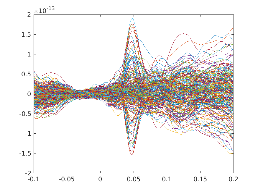
We can plot the results with the MATLAB plot command to get a first impression

figure; plot(timelock.time, timelock.avg)

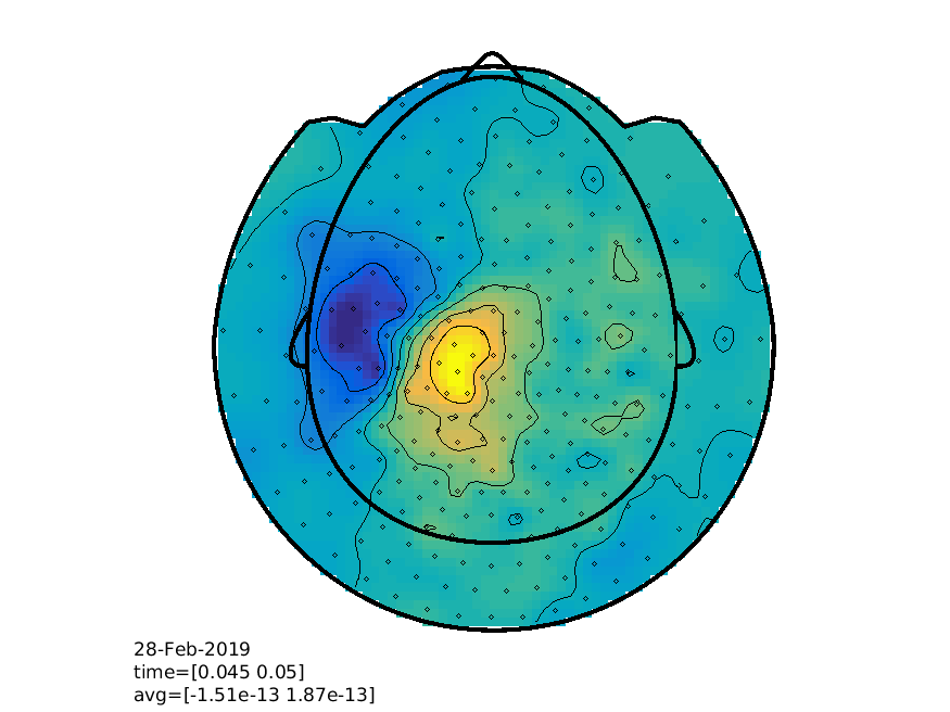
We can additionally explore the spatiotemporal dynamics using FieldTrip interactive plotting function

% view the results
cfg        = [];
cfg.layout = 'CTF275_helmet.mat';
cfg.xlim   = [0.045 0.050];
ft_topoplotER(cfg, timelock);

Visualize the sensor level results (planar gradients)

The present dataset was recorded with a CTF MEG system which has first-order axial gradiometer sensors that measure the gradient of the magnetic field in the radial direction, i.e. orthogonal to the scalp. Often it is helpful to interpret the MEG fields after transforming the data to a planar gradient configuration, i.e. by computing the gradient tangential to the scalp. This representation of MEG data is comparable to the field measured by planar gradiometer sensors. One advantage of the planar gradient transformation is that the signal amplitude typically is largest directly above a source.

With ft_megplanar we calculate the planar gradient of the averaged data. Ft_combineplanar is used to compute the magnitude of the planar gradient by combining the horizontal and vertical components of the planar gradient;

The planar gradient at a given sensor location can be approximated by comparing the field at that sensor with its neighbours (i.e. finite difference estimate of the derivative). The planar gradient at one location is computed in both the horizontal and the vertical direction with the FieldTrip function ft_megplanar. These two orthogonal gradients on a single sensor location can be combined using Pythagoras rule with the FieldTrip function ft_combineplanar.

Calculate the planar gradient of the averaged dat

% calculate planar gradients
cfg                 = [];
cfg.feedback        = 'yes';
cfg.method          = 'template';
cfg.template        = 'ctf275_neighb.mat';
cfg.neighbours      = ft_prepare_neighbours(cfg, timelock);

cfg.planarmethod    = 'sincos';
timelock_planar     = ft_megplanar(cfg, timelock);

Compute the amplitude of the planar gradient by combining the horizontal and vertical components of the planar gradient according to Pythagoras rule, and visualize the results (can you see the differences between the axial and planar gradients?

% combine planar gradients
cfg                 = [];
timelock_planarcomb = ft_combineplanar(cfg, timelock_planar);

% view the results
cfg        = [];
cfg.layout = 'CTF275_helmet.mat';
cfg.xlim   = [0.045 0.050];
ft_topoplotER(cfg, timelock_planarcomb);

The forward model and lead field matrix

Head model

The first step in the procedure is to construct a forward model. The forward model allows us to calculate an estimate of the field measured by the MEG sensors for a given current distribution. In MEG analysis a forward model is typically constructed for each subject. There are many types of forward models which to various degrees take the individual anatomy into account. We will here use a semi-realistic head model developed by Nolte (2003). It is based on a correction of the lead field for a spherical volume conductor by a superposition of basis functions, gradients of harmonic functions constructed from spherical harmonics.

The first step in constructing the forward model is to find the brain surface from the subject’s MRI, using ft_volumesegment. The MRI scan used in this tutorial has already been realigned to the same coordinate system as the MEG data (in this case ‘CTF’, see this page on how to realign your subject’s brain volume.

% read and segment the subject's anatomical scan
load('SubjectSEF_mri.mat'); % matfile containing the realigned anatomical scan

cfg        = [];
cfg.output = 'brain';
seg = ft_volumesegment(cfg, mri);

% make a figure of the mri and segmented volumes
segmentedmri           = seg;
segmentedmri.transform = mri.transform;
segmentedmri.anatomy   = mri.anatomy;
cfg                    = [];
cfg.funparameter       = 'brain';
ft_sourceplot(cfg, segmentedmri);

Now prepare the head model from the segmented brain surface:

% compute the subject's headmodel/volume conductor model
cfg                = [];
cfg.method         = 'singleshell';
headmodel          = ft_prepare_headmodel(cfg, seg);
headmodel          = ft_convert_units(headmodel, 'cm'); % mm to cm, just to be sure

Source model

Now prepare the source model. Here one has the option to make a ‘normalized grid’, such that the grid points in different subjects are aligned in MNI-space. For more details on how to make a normalized grid, see here. In this tutorial, we continue with non-normalized grid points:

% create the subject specific grid
grad = ft_read_sens('SubjectSEF.ds', 'senstype', 'meg');

cfg             = [];
cfg.grad        = grad;
cfg.headmodel   = headmodel;
cfg.resolution  = 0.5;
cfg.inwardshift = -1;
sourcemodel     = ft_prepare_sourcemodel(cfg);

% make a figure of the single subject headmodel, and grid positions
figure;
ft_plot_sens(grad, 'style', '*b');
ft_plot_headmodel(headmodel, 'edgecolor', 'none'); alpha 0.4;
ft_plot_mesh(sourcemodel.pos(sourcemodel.inside,:));

Leadfield

Combine all the information into the leadfield matrix:

% create leadfield
cfg                  = [];
cfg.grad             = grad;  % gradiometer distances
cfg.headmodel        = headmodel;   % volume conduction headmodel
cfg.sourcemodel      = sourcemodel;
cfg.channel          = {'MEG'};
cfg.singleshell.batchsize = 2000;
lf                   = ft_prepare_leadfield(cfg);

Source analysis

% create spatial filter using the lcmv beamformer
cfg                  = [];
cfg.method           = 'lcmv';
cfg.sourcemodel      = lf; % leadfield
cfg.headmodel        = headmodel; % volume conduction model (headmodel)
cfg.lcmv.keepfilter  = 'yes';
cfg.lcmv.fixedori    = 'yes'; % project on axis of most variance using SVD
source               = ft_sourceanalysis(cfg, timelock);